PhD Research: Methodological Developments
My doctoral research developed computational methods to process, analyse and visualise complex architectural and urban data from disparate sources to build a more robust multi faceted understanding of spatial conditions.
Corrective Geometric Analysis
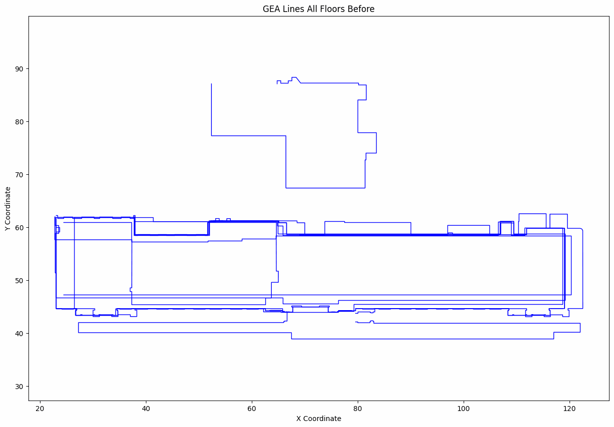
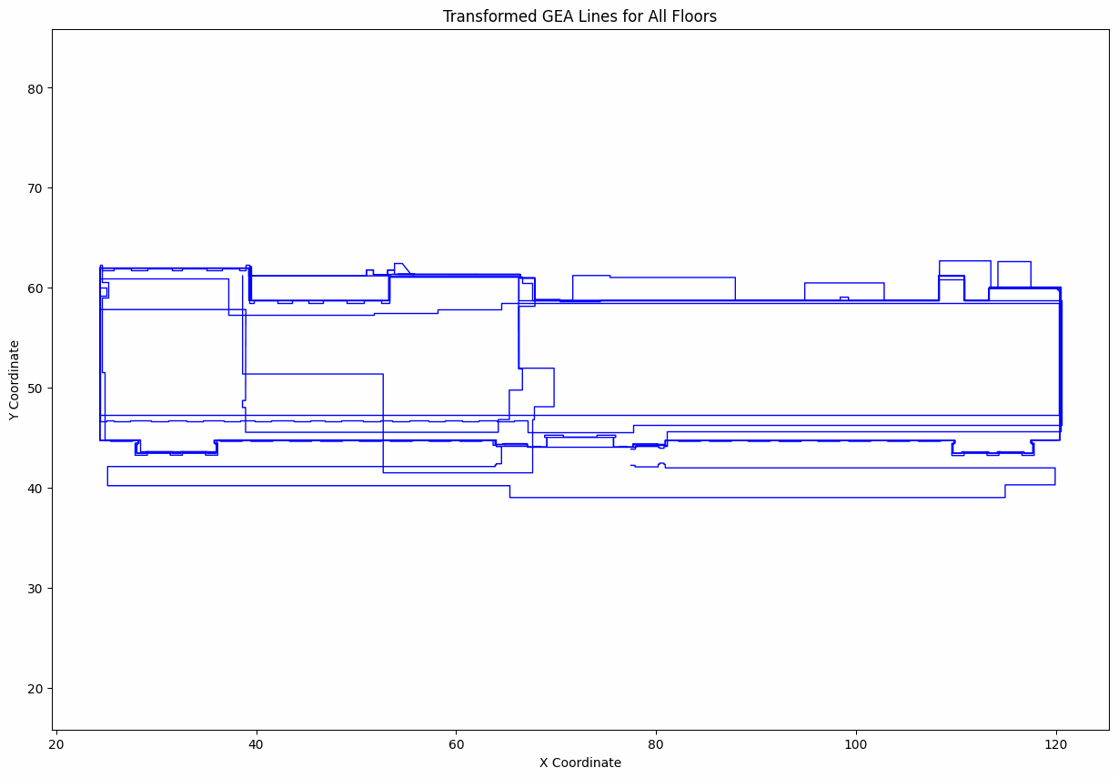
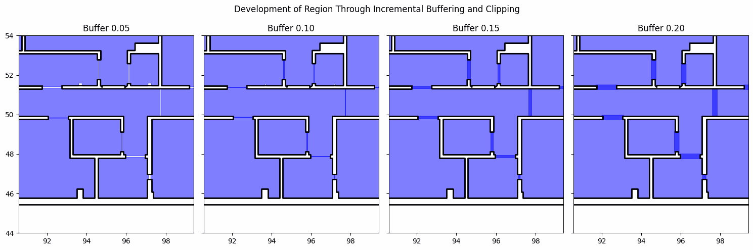
Pipeline for cleaning raw inconsistent floorplan vector data and preparing it for downstream analysis and modelling. The left figure highlights minute fissures within the digital geometry, subtle gaps and breaks that had to be repaired before the dataset could be reliably used. The right figure shows misalignment across floors requiring rectification. I implemented custom routines to repair gaps, snap endpoints and normalise topology so the data became stable for further spatial analysis.
Hover to magnify repaired micro‑gaps (red) originating from stray vertices (yellow). Scroll to zoom.
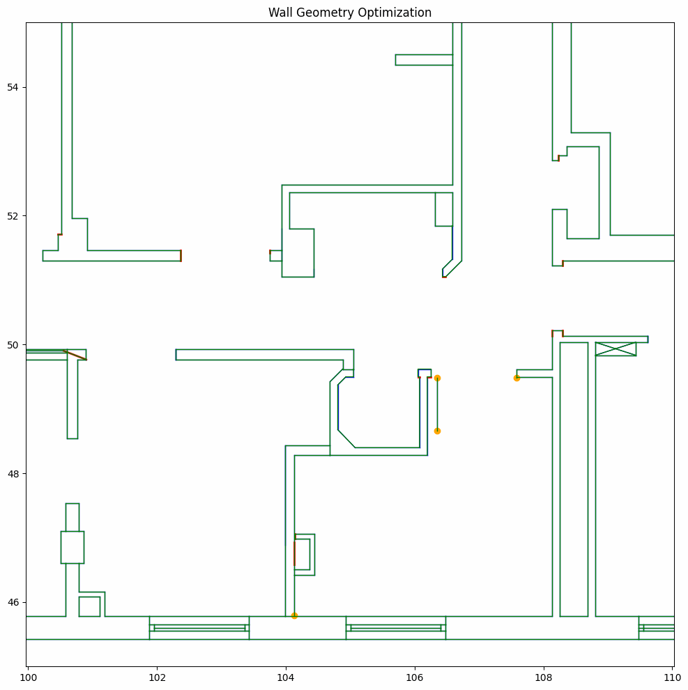
Drag the slider to compare original unaligned vs. aligned floorplate outlines.
Spatial Analysis: Adjacency and VGA Integration
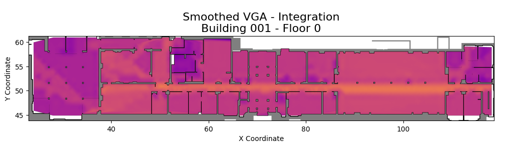
Expansion and clipping strategies infer doorless adjacencies and construct a connectivity graph, shown by inflated room polygons. Alongside, Visibility Graph Analysis (VGA) highlights global and local integration values. Together these views show how configuration and connectivity influence potential movement and accessibility within the plan.
From Local Drawing to Global Context
Relating indoor geometry to geographic reference frames enables multi scale spatial reasoning. The task is to align CAD native local coordinates to a projected global footprint while preserving geometry. This section outlines that registration.
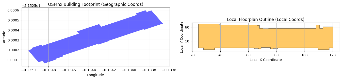
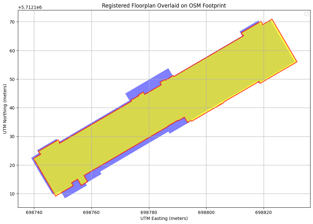
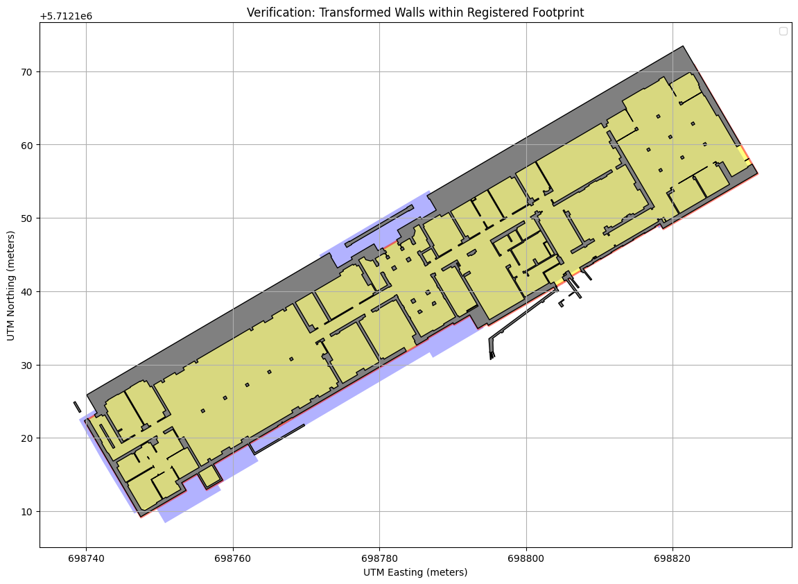
Mathematical Registration and Transformation Matrix
Goal: derive a single stable affine 3×3 matrix mapping any local CAD floorplan coordinate into a projected global metric frame (UTM) so every downstream geometry (walls, cameras, analysis overlays) can be reproduced deterministically.
Local geometry → (T-Clocal) → (Uniform scale s) → (Rotate θ) → (Translate to CUTM) → (ICP refine Δθ, Δt) → Global geometry
Stage 1 · Coordinate System & PCA Alignment
- Projection: The OSM footprint (EPSG:4326) is projected to its appropriate UTM zone chosen from the footprint centroid (automatic CRS estimation).
- Principal axis extraction: Both the projected footprint and the local floorplan obtain a minimum rotated rectangle (MRR); the longest edge gives a dominant axis length L and orientation θ (computed from that edge vector).
- Scale: s = Lutm / Llocal (strictly uniform). Derived: s = 1.0030 (metres per local unit).
- Rotation: θ = θutm - θlocal. Derived: θ = -149.20°.
- Translation: shift centroid Clocal → CUTM. Derived: Clocal = (70.52, 52.61), CUTM = (698784.56, 5712139.76).
Operations are applied about the origin for numerical stability: translate to origin → scale → rotate → translate to CUTM. This yields the preliminary matrix Mpca.
Stage 2 · ICP Refinement (Rotation + Translation Only)
- Input: Vertices of the already aligned polygon (after Stage 1) and vertices of the projected footprint.
- Nearest-neighbour model: A KD‑tree (cKDTree) over target vertices supplies fast closest-point queries (vertex-to-vertex approximation).
- Optimisation: L‑BFGS‑B minimises the sum of squared nearest‑neighbour distances over parameters [Δtx, Δty, Δθ, scale]. Bounds lock scale = 1.0 (no further dilation).
- Result: corrective pose: Δt = (2.159, 1.225) m, Δθicp = -0.472°, scale fixed at 1.000.
Because scale is fixed, refinement cannot accidentally introduce aspect drift; only rigid pose is nudged to minimise residual misalignment.
Matrix Composition
Matrix multiplication is evaluated right → left. All matrices are 3×3 homogeneous transforms, enabling a single pass over any set of 2D coordinates augmented with 1.
Action on a Point
Linear part encodes combined rotation + uniform scale; translation column encodes global placement. Because scaling/rotation were performed about the centroid (after origin shift) distortion is minimised and numerical stability preserved.
Parameter Derivation Summary
- s (scale): 1.0030 (dominant axis length ratio).
- θ (rotation): -149.20° (principal axis difference).
- Centroids: Clocal = (70.52, 52.61), CUTM = (698784.56, 5712139.76).
- ICP correction: Δθicp = -0.472°, Δt = (2.159, 1.225) m, scale held at 1.000.
Final Matrix (Linear Part & Consistency)
[[ -0.865674649   0.506515064   698821.116 ]
 [ -0.506515064  -0.865674649  5712222.225 ]
 [  0.000000000   0.000000000     1.000000 ]]
[[  s cosθᵗ    -s sinθᵗ     tₓ  ]
 [  s sinθᵗ     s cosθᵗ     tᵧ  ]
 [    0            0         1  ]]
θᵗ = θ + Δθicp = −149.20° + (−0.472°) = −149.672°
s = 1.0030 → ‖first column‖ ≈ 1.003 (uniform scale)
t = (698821.116 , 5712222.225) m (global translation)
Linear block (top-left 2×2) encodes uniform scale + cumulative rotation θᵗ; determinant ≈ s² confirms no shear.
The resulting Mfinal is applied uniformly to all subsequent geometries (e.g. multi‑polygon wall sets) ensuring deterministic georeferencing across the pipeline.
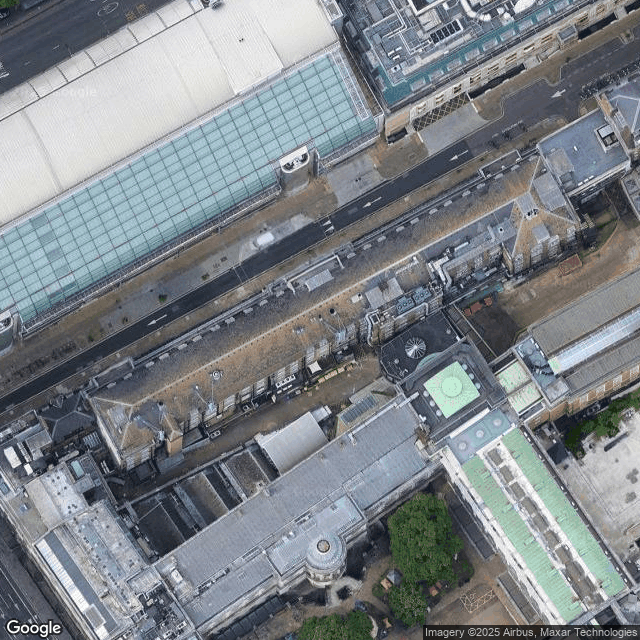
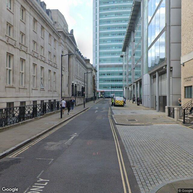
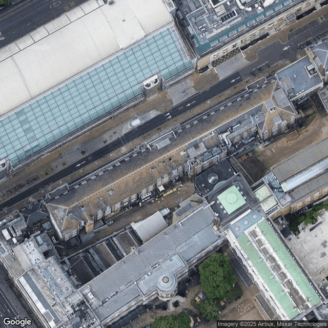
Imagery Acquisition and Camera Interpolation
Imagery from multiple sources is acquired for the registered case study (Kathleen Lonsdale Building). Satellite and Street View images are obtained via Google Maps APIs and georeferenced using the OSMx pathway. Using both perspectives I interpolate between camera poses. Limitations of manual keyframe definition in Google Earth Studio led me to reverse engineer the save file format to define projects programmatically enabling smooth controlled interpolation. The GIF shows a continuous transition.
Automation Pipeline: From Data to 3D Scene
A fully automated pipeline constructs a multi storey 3D model from raw 2D geometry. Stage one (Python) sorts complex floor levels including basements mezzanines and roofs, applies the affine transformation matrix to georeference geometry, assumes a nominal 3 m floor to floor height unless specified and serialises camera data to JSON.
Stage two (Blender) reconstructs the scene from JSON using the bmesh API for mesh creation, builds each floor at the correct elevation, applies basic materials and sets up all registered camera views and lighting. The process is repeatable and deterministic.
1. Python: Data Preparation
# --- Data Preparation & Georeferencing ---
# This script defines a pipeline to process raw architectural data (including
# complex floor levels) and georeferenced cameras, transforming them into
# a clean, structured, and localized 3D scene format for Blender.

import numpy as np
import geopandas as gpd
from shapely.geometry import Point
from shapely.affinity import apply as apply_transform
from geopy.distance import geodesic

# Define a constant for story height
FLOOR_HEIGHT = 3.0

# Define the final output path.
# This path should match the JSON_FILEPATH variable in your Blender script.
JSON_FILEPATH = "/path/to/blender_scene_data_all.json"

def sort_floor_keys(floors_dict):
    """
    Robustly sorts complex floor keys (e.g., '-1', '0', '2.5', 'R') into
    a logical vertical stack based on numeric value and special rules.
    """
    floor_map = []
    # Logic to parse numeric and special string keys like 'R' for Roof...
    numeric_keys = [float(k) for k in floors_dict if k.replace('.', '', 1).replace('-', '', 1).isdigit()]
    max_numeric_index = max(numeric_keys) if numeric_keys else -1

    for key in floors_dict.keys():
        try:
            numeric_index = float(key)
        except ValueError:
            numeric_index = max_numeric_index + 1 if key.upper() == 'R' else None

        if numeric_index is not None:
            floor_map.append({'original_key': key, 'numeric_index': numeric_index})

    return sorted(floor_map, key=lambda x: x['numeric_index'])

def prepare_data_for_blender(building_footprint, building_structure, selected_cameras_gdf, target_utm_crs, final_matrix):
    """
    Main function to orchestrate the data preparation pipeline.
    """
    # 1. Establish a local 3D origin from the building's projected centroid.
    local_origin = building_footprint.centroid
    origin_x, origin_y = local_origin.x, local_origin.y

    blender_data = {"building_geometries": [], "cameras": []}

    # 2. Sort all floor levels into a logical vertical order.
    sorted_floors = sort_floor_keys(building_structure['001']['floors'])

    # 3. Process each floor's geometry.
    for floor_info in sorted_floors:
        floor_data = building_structure['001']['floors'][floor_info['original_key']]
        base_z = floor_info['numeric_index'] * FLOOR_HEIGHT

        for wall_poly in floor_data.get('wall_polygon').geoms:
            # 3a. Apply a pre-calculated affine transformation matrix to align geometry.
            transformed_wall = apply_transform(wall_poly, final_matrix)

            # 3b. Re-center vertex coordinates relative to the local origin.
            verts_utm = np.array(transformed_wall.exterior.coords)
            local_verts = (verts_utm - [origin_x, origin_y]).tolist()

            blender_data["building_geometries"].append({
                "name": f"Wall_F{floor_info['original_key']}", "base_z": base_z, "verts": local_verts
            })

    # 4. Process and re-center each selected Street View camera.
    for index, cam_data in selected_cameras_gdf.iterrows():
        cam_point_geo = cam_data.geometry
        cam_heading = cam_data['original_heading']

        # 4a. Project camera's geographic lat/lon to the scene's projected UTM CRS.
        cam_point_utm = gpd.GeoSeries([cam_point_geo], crs="EPSG:4326").to_crs(target_utm_crs).iloc[0]
        cam_pos_utm = np.array([cam_point_utm.x, cam_point_utm.y, 2.5]) # Assume 2.5m camera height

        # 4b. Calculate a target point 10m away to define camera's viewing direction.
        target_geo_point = geodesic(meters=10).destination((cam_point_geo.y, cam_point_geo.x), cam_heading)
        target_utm_point = gpd.GeoSeries([Point(target_geo_point.longitude, target_geo_point.latitude)], crs="EPSG:4326").to_crs(target_utm_crs).iloc[0]
        target_pos_utm = np.array([target_utm_point.x, target_utm_point.y, 2.5])

        # 4c. Re-center 3D camera position and target relative to the local origin.
        local_cam_pos = (cam_pos_utm - [origin_x, origin_y, 0]).tolist()
        local_target_pos = (target_pos_utm - [origin_x, origin_y, 0]).tolist()

        blender_data["cameras"].append({
            "name": f"StreetView_Cam_h{int(cam_heading)}", "pos": local_cam_pos, "target": local_target_pos
        })

    return blender_data

# --- Implementation ---

# 1. Load the building's raw footprint and apply the transformation matrix
#    to create the final, registered footprint ('final_registered_fp').
final_registered_fp = apply_transformation_matrix(raw_footprint, final_matrix)

# 2. Load the full building data structure from a pre-processed pickle file.
sorted_building_structure = load_pickle_data("path/to/data.pickle")

# 3. Load the GeoDataFrame containing all potential camera positions and their
#    metadata, as returned by the Street View API analysis.
locations_gdf = gpd.read_file("path/to/camera_locations.geojson")

# 4. Filter for the specific cameras to be exported to the 3D scene.
desired_headings = [237, 135, 86]
selected_cameras_gdf = locations_gdf[locations_gdf['original_heading'].isin(desired_headings)]

# 5. Run the main function to generate the structured JSON for Blender.
blender_scene_data = prepare_data_for_blender(
    final_registered_fp,
    sorted_building_structure,
    selected_cameras_gdf,
    utm_crs, # The target CRS object (e.g., from the registered footprint)
    final_matrix
)

# 6. Save the prepared data to the target JSON file.
with open(JSON_FILEPATH, 'w') as f:
    json.dump(blender_scene_data, f, indent=4)
2. Blender: 3D Reconstruction
# --- 3D Scene Reconstruction (Blender `bpy`) ---
# This script reads a structured JSON file and programmatically
# reconstructs a complete, multi-story 3D architectural scene with
# georeferenced cameras and a sample lighting setup.

import bpy
import bmesh
import json
import math

# Define input path.
JSON_FILEPATH = "/path/to/blender_scene_data_all.json"

WALL_HEIGHT = 3.0

# --- Helper Function: Geometry Creation ---
def create_mesh_wall(name, verts_2d, interiors_2d=[], base_z=0.0):
    """
    Efficiently creates a 3D wall mesh from 2D vertex data using the bmesh API.
    Handles complex polygons with interior holes.
    """
    mesh = bpy.data.meshes.new(name + "_data")
    obj = bpy.data.objects.new(name, mesh)
    bpy.context.collection.objects.link(obj)
    bm = bmesh.new()

    # Create the 2D base face, including any holes
    verts_at_zero = [bm.verts.new((v[0], v[1], 0)) for v in verts_2d]
    base_face = bm.faces.new(verts_at_zero)
    for hole_verts_2d in interiors_2d:
        hole_verts = [bm.verts.new(v) for v in hole_verts_2d]
        bmesh.ops.delete(bm, geom=[bm.faces.new(hole_verts)], context='FACES')

    # Extrude the face region vertically to create a solid wall
    extruded = bmesh.ops.extrude_face_region(bm, geom=[base_face])
    extruded_verts = [v for v in extruded['geom'] if isinstance(v, bmesh.types.BMVert)]
    bmesh.ops.translate(bm, verts=extruded_verts, vec=(0, 0, WALL_HEIGHT))

    bm.to_mesh(mesh)
    bm.free()
    obj.location.z = base_z
    mesh.update()

# --- Helper Function: Camera Creation ---
def create_camera_with_target(name, pos, target_pos):
    """
    Creates a new camera and an 'Empty' object to serve as its target,
    then uses a 'Track To' constraint to ensure it is aimed correctly.
    """
    target = bpy.data.objects.new(name + "_target", None)
    target.location = target_pos
    bpy.context.collection.objects.link(target)

    cam_data = bpy.data.cameras.new(name)
    cam_obj = bpy.data.objects.new(name, cam_data)
    cam_obj.location = pos
    bpy.context.collection.objects.link(cam_obj)

    constraint = cam_obj.constraints.new(type='TRACK_TO')
    constraint.target = target

# --- Main Orchestration Function ---
def main():
    # 1. Load the prepared scene data from the JSON file.
    with open(JSON_FILEPATH, 'r') as f:
        scene_data = json.load(f)

    # 2. Procedurally set up a sample lighting environment.
    setup_lighting() # Creates sun and ambient world light

    # 3. Iterate through geometry data to build the multi-story building.
    for geom_data in scene_data.get("building_geometries", []):
        create_mesh_wall(
            name=geom_data.get("name"),
            verts_2d=geom_data.get("verts"),
            interiors_2d=geom_data.get("interiors", []),
            base_z=geom_data.get("base_z")
        )

    # 4. Iterate through camera data to place and aim virtual cameras.
    for cam_data in scene_data.get("cameras", []):
        create_camera_with_target(
            name=cam_data.get("name"),
            pos=cam_data.get("pos"),
            target_pos=cam_data.get("target")
        )

    print("Blender scene reconstruction complete!")

# --- Script Execution ---
if __name__ == "__main__":
    main()
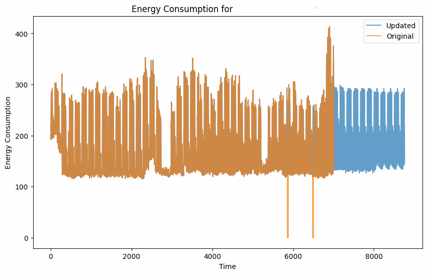
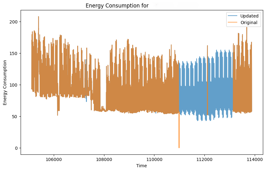
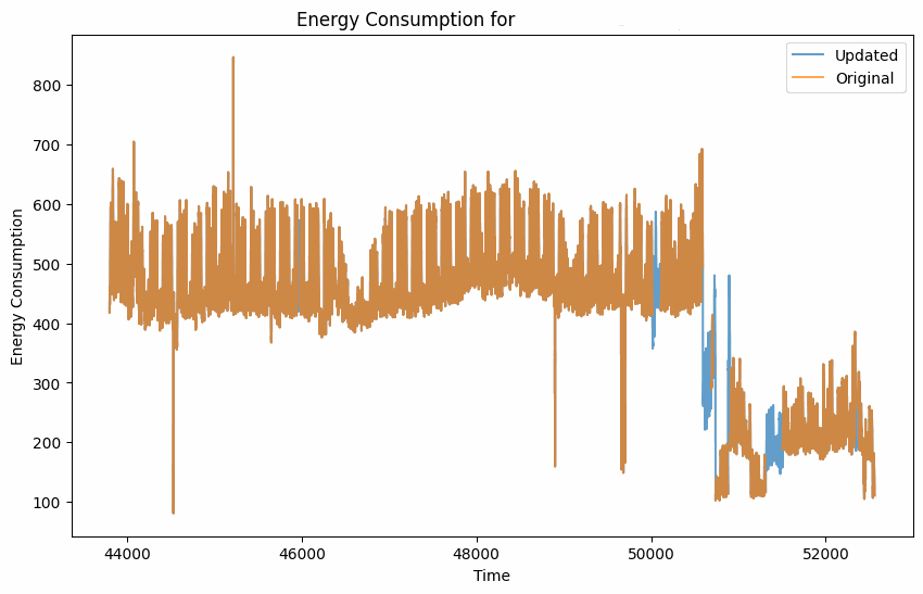
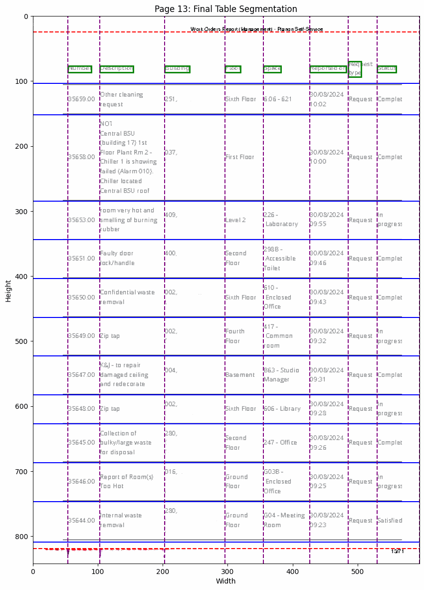
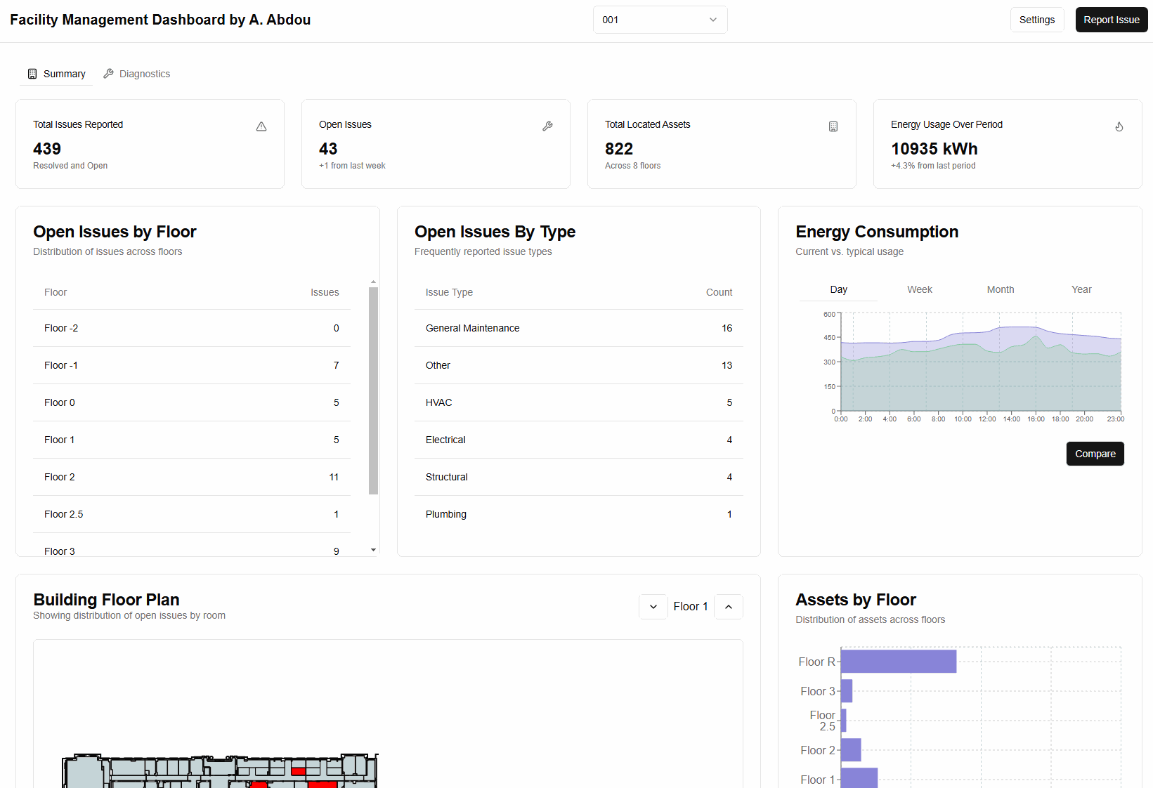
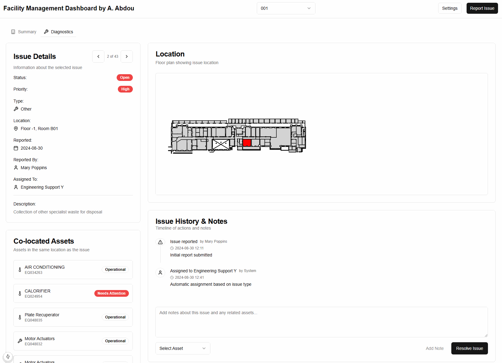
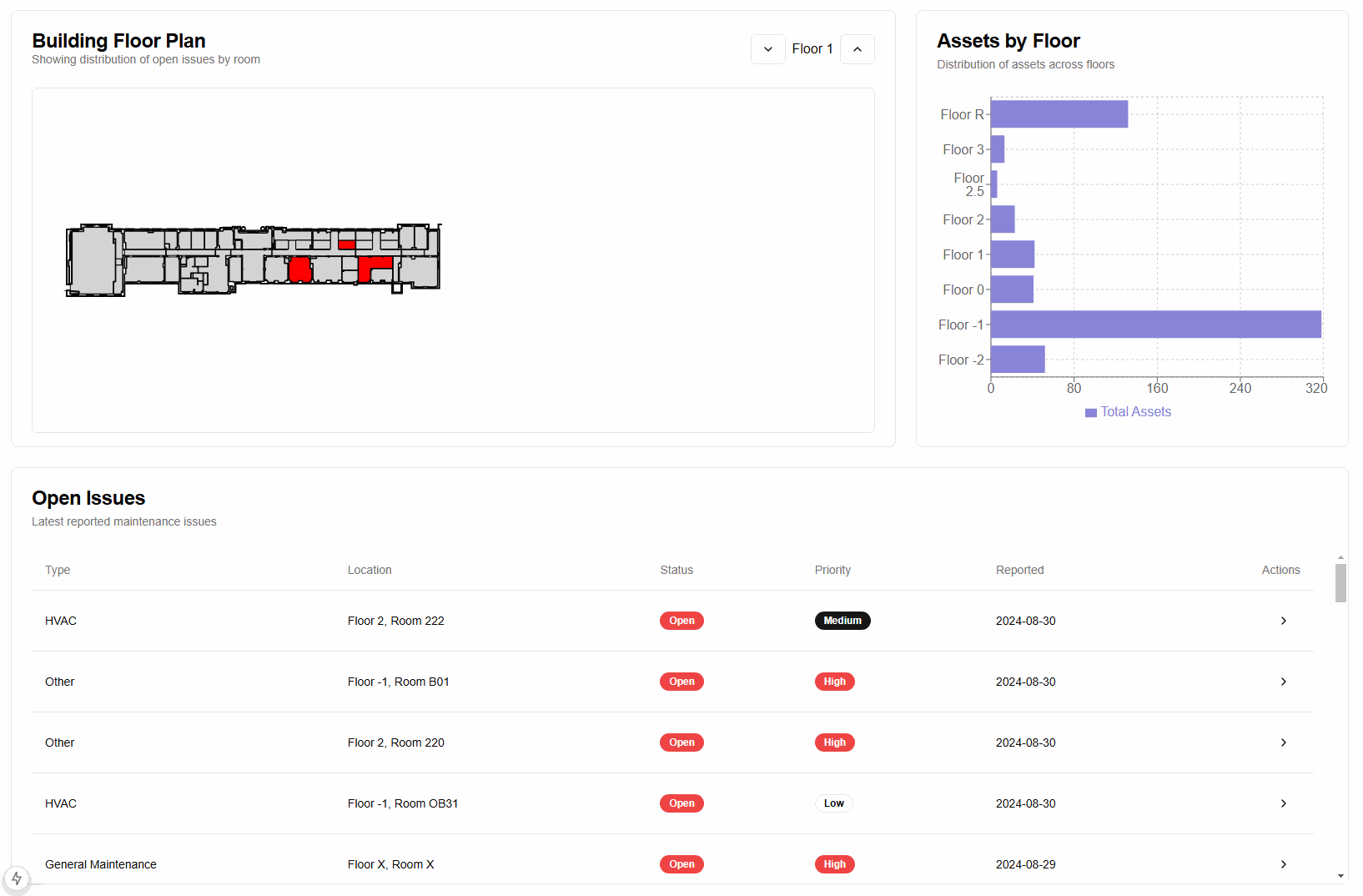
Supporting Methodological Toolkit
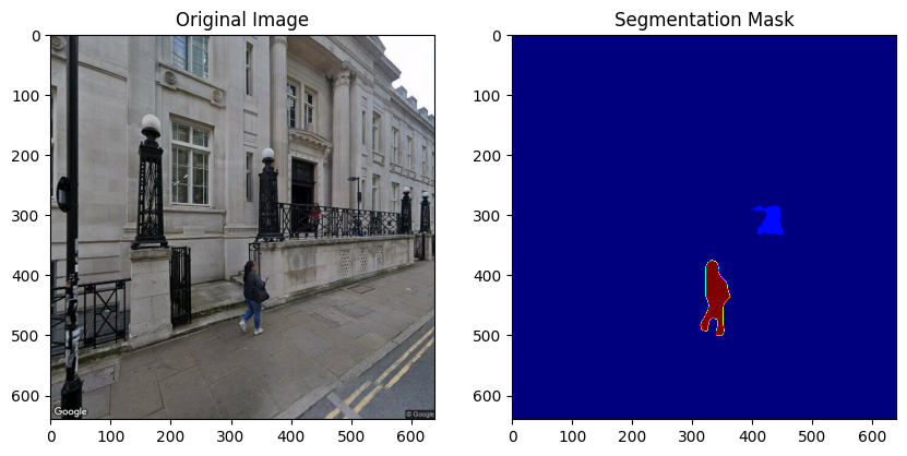
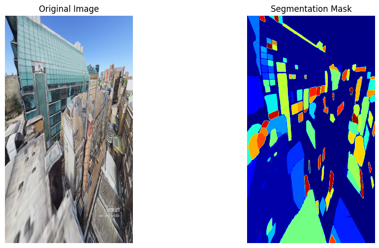
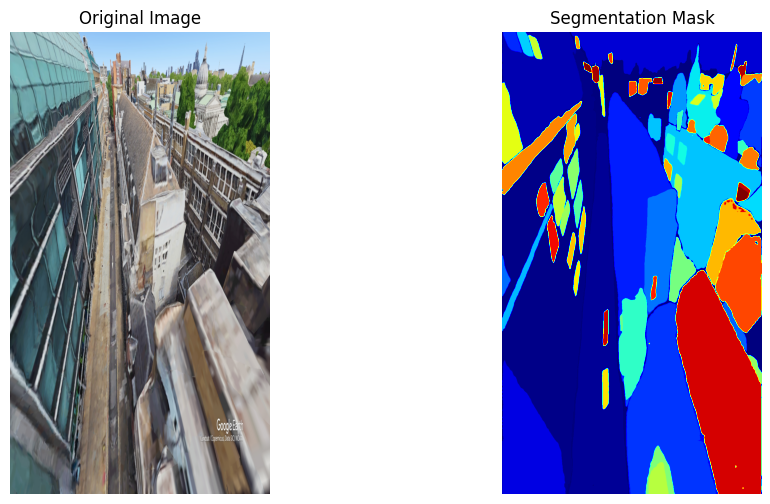
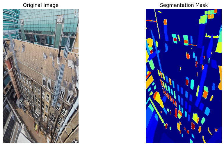
Complementary utilities: ML based energy data imputation, PDF structure parser, integrated analytics dashboard and experimental semantic segmentation (SAM) on generated imagery.